Tensorflow 2 Object Detection API Tutorial with a GPU in Windows 10

Hello there! Today I will be completing the Tensorflow 2 Object Detection API Tutorial on my new Windows PC.

I have already set up my development environment so I can already run Tensorflow 2.4 with Python 3.8 and using Anaconda. Also, I have added GPU support to Tensorflow because I have installed all the Nvidia CUDA libraries, including cuDNN.

If you haven’t set up yet your development environment, I recommend you to read this guide or if you prefer watch my video where I complete the setup:

Without further ado let’s get started!

If you haven’t set up yet your development environment, I recommend you to read this guide or if you prefer watch my video where I complete the setup:

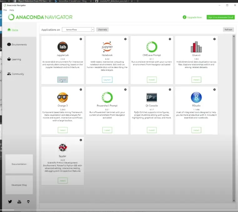
Starting Anaconda Navigator

Select Home and click on the dropdown, and choose the Tensorflow environment that we created in the last video.

This Anaconda environment already has all the libraries needed to run Tensorflow 2.4 with GPU support.

Starting JupyterLab

Click Launch under the JupyterLab icon. A new browser window will be automatically opened with JupyterLab.

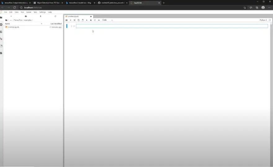
This is going to be where we will do all our Python and Tensorflow development.

JupyterLab. is a very useful web-based IDE for Python and is highly favored by Data Scientists as a way of sharing live code using simple notebooks. And today we will find out why they are so popular.

Testing that the Tensorflow module is available

First I am going to check that the tensorflow python library is available:

[] import tensorflow

Since I get no errors, we are good to go.

Object Detection API with Static Images

Now that we know that Tensorflow works, we will try Object Detection API against static images using models from the model zoo in the Tensorflow Github repository.

What is the model Zoo?

The model zoo is a collection of pre-trained models by Google trained on the COCO 2017 dataset of images. The COCO 2017 dataset is a collection of over 120k labelled images.

A labelled image is one in which an image has annotations which explain what the image contain. This is very useful for training object detection models.

Transfer Learning

These models can be immediately used to identify objects for which they have already been trained to identify(inference) or can be trained further using Transfer Learning.

I will not go too much into detail about Transfer Learning for now. Suffice to know, it can take a lot of time, training data, and money to train a model from scratch, and with Transfer Learning it is possible to cheap out.

For example if we know a pre-trained model can detect animals in general, we can use Transfer Learning and a little bit of extra data to teach the AI model to differentiate Lions from Leopards.

Model Zoo Metrics

As you can see the model zoo table has quite a few models available. All these models have slightly different architectures, which can be identified by the names.

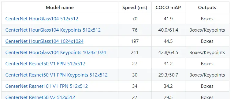
First in the list is CenterNet, an architecture which represents objects as points, rather than bounding boxes coordinates as most typical architectures do.

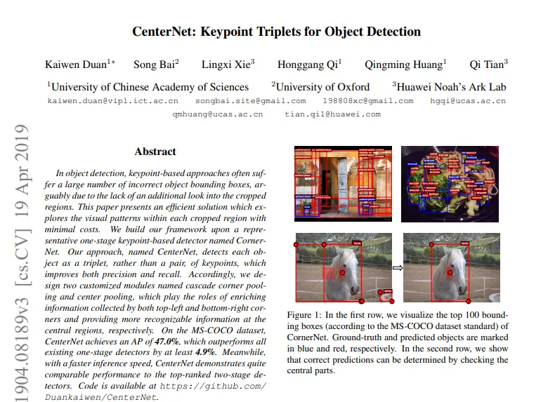
This was an advance in object detection frameworks because it allowed the object detection to be more accurate and faster than other models which use bounding boxes.

Further down the list we can see more models belonging to the EfficientDet architecture. This architecture is also a new recent development, a successor to Efficient, coming out from the Google Brain labs in July 2020, which require less training epochs and less compute power to do inferencing. It is more accurate and much faster than previous architectures such as YOLOv3, RetinaNet and Mask R-CNN.

As you can see there are a lot of models to choose from. Therefore we need to understand the metrics available, so we pick the best model for our use-case.

Speed(Ms)

This is the expected response time to get a response when querying the model. This metric doesn’t include the time it takes to load the model into memory, since that is usually done only once.

The lower the better.

COCO mAP

The mean average precision score against the COCO dataset of images. The higher value, the better.

The input image size

Next to each model name we can see the images sizes, for example:

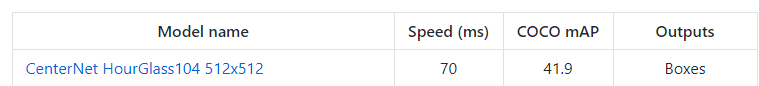
Here I am making assumptions since the documentation doesn’t explain any further. The 512×512 is the input image size that this model has been trained with. What that means is that when you call this model with an image, the image will be resized to 512×512.

Looking at the metrics, I can see that the mAP increases with input image size, but the Speed(ms) increases as well. If you are looking to do near real-time inference you will need to do a trade-off between speed and accuracy.

Trying the Tensorflow 2 Object Detection Example in the documentation

Now that we have a better understanding of the Tensorflow Model Zoo, we can start copy and pasting code for our first example.

import os
os.environ['TF_CPP_MIN_LOG_LEVEL'] = '2'    # Suppress TensorFlow logging (1)
import pathlib
import tensorflow as tf

tf.get_logger().setLevel('ERROR')           # Suppress TensorFlow logging (2)

# Enable GPU dynamic memory allocation
gpus = tf.config.experimental.list_physical_devices('GPU')
for gpu in gpus:
    tf.config.experimental.set_memory_growth(gpu, True)

def download_images():
    base_url = 'https://raw.githubusercontent.com/tensorflow/models/master/research/object_detection/test_images/'
    filenames = ['image1.jpg', 'image2.jpg']
    image_paths = []
    for filename in filenames:
        image_path = tf.keras.utils.get_file(fname=filename,
                                            origin=base_url + filename,
                                            untar=False)
        image_path = pathlib.Path(image_path)
        image_paths.append(str(image_path))
    return image_paths

IMAGE_PATHS = download_images()

This first block of code seems to be suppressing any excess logging that Tensorflow will throw at us by default and there seems to be a if statement just for GPUs:

# Enable GPU dynamic memory allocation
gpus = tf.config.experimental.list_physical_devices('GPU')
for gpu in gpus:
    tf.config.experimental.set_memory_growth(gpu, True)

This if statement, seems to be resolving previous issues with Tensorflow 1.x where one could run out of memory in the GPU because all memory was allocated at the beginning. Not really important today, but it is useful to keep this setting in mind in case for the future.

More straightforward to understand, we are also downloading the test images from the Tensorflow github repository!

Downloading the Model

# Download and extract model
def download_model(model_name, model_date):
    base_url = 'http://download.tensorflow.org/models/object_detection/tf2/'
    model_file = model_name + '.tar.gz'
    model_dir = tf.keras.utils.get_file(fname=model_name,
                                        origin=base_url + model_date + '/' + model_file,
                                        untar=True)
    return str(model_dir)

MODEL_DATE = '20200711'
MODEL_NAME = 'centernet_hg104_1024x1024_coco17_tpu-32'
PATH_TO_MODEL_DIR = download_model(MODEL_NAME, MODEL_DATE)

We are downloading the ‘centernet_hg104_1024x1024_coco17_tpu-32’ model.

This model uses the CenterNet architecture and it accepts input images with resolution of 1024×1024.

We are using a Keras utility function(tf.keras.utils.get_file) to download the model.

Downloading the COCO Dataset Labels

The model we downloaded in the previous step was trained using the COCO dataset. When we call the model for inference, this model will only return the id(number) of each object class identified. It is missing the label.

In order to know what these object classes are, we need to download the COCO dataset labels:

# Download labels file
def download_labels(filename):
    base_url = 'https://raw.githubusercontent.com/tensorflow/models/master/research/object_detection/data/'
    label_dir = tf.keras.utils.get_file(fname=filename,
                                        origin=base_url + filename,
                                        untar=False)
    label_dir = pathlib.Path(label_dir)
    return str(label_dir)

LABEL_FILENAME = 'mscoco_label_map.pbtxt'
PATH_TO_LABELS = download_labels(LABEL_FILENAME)

You can see below an example of how labels are stored in this text file:

item {
  name: "/m/01g317"
  id: 1
  display_name: "person"
}

Using the label above as an example, if the object detection API finds any objects in an image with identifier id =1 then the label will be set to person.

Loading the Model

import time
from object_detection.utils import label_map_util
from object_detection.utils import visualization_utils as viz_utils

PATH_TO_SAVED_MODEL = PATH_TO_MODEL_DIR + "/saved_model"

print('Loading model...', end='')
start_time = time.time()

# Load saved model and build the detection function
detect_fn = tf.saved_model.load(PATH_TO_SAVED_MODEL)

end_time = time.time()
elapsed_time = end_time - start_time
print('Done! Took {} seconds'.format(elapsed_time))

Now that we have downloaded the labels, it is to time to load the model into memory.

It might take a while to load into memory.

Let’s take a look at the model that we downloaded.

The saved model used in this example is large! The file compressed is 1.4GB.

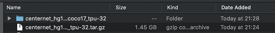
And uncompressed, about 1.6GB.

Inside the model directory, we can see two folders:

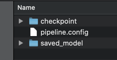
The saved_model directory and the checkpoint folder.

The checkpoint folder contains the following files:

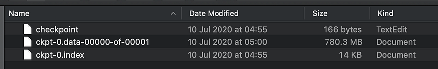
ckpt-0.data-00000–of-00001 contains the trained weights needed to resume training the model if we wished to. Note that ckpt-0.index is the file that indicates which weights are stored in which file. If there were more than one shard we would have multiple ckpt-0.data-x–of-Y files.

More interesting is the content of the checkpoint file:

model_checkpoint_path: "ckpt-0"
all_model_checkpoint_paths: "ckpt-0"
all_model_checkpoint_timestamps: 1594334668.5972695
last_preserved_timestamp: 1594334661.7811196

The above timestamp tells me that this checkpoint was created on the 9th of July 2020!

The saved_model directory contains the following files:

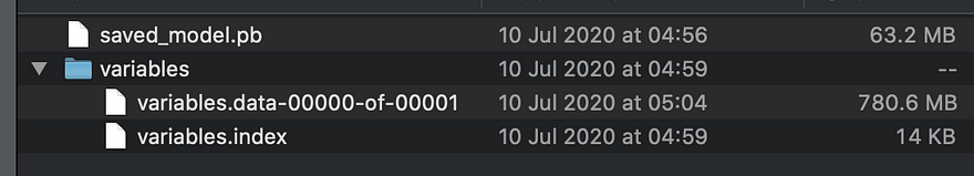
saved_model.pb

The saved_model.pb file is in protobuf binary format and stores the model code and a set of function signatures that the model accepts.

The weights for the model are stored inside the variables directory. The big file here seems to be the weights(variables.data-00000–of-00001.

After 140s the model finally is loaded into memory. Not bad considering the size of the files!

Mapping between category index and labels

category_index = label_map_util.create_category_index_from_labelmap(PATH_TO_LABELS,use_display_name=True)

Using the label map we downloaded earlier and a utility function that comes with the object detection API we create a dictionary that maps an object class id, or as it is called here category index, to a label.

Loading an image into a NumPy array

import numpy as np
from PIL import Image
import matplotlib.pyplot as plt
import warnings
warnings.filterwarnings('ignore')   # Suppress Matplotlib warnings

def load_image_into_numpy_array(path):
    """Load an image from file into a numpy array.

    Puts image into numpy array to feed into tensorflow graph.
    Note that by convention we put it into a numpy array with shape
    (height, width, channels), where channels=3 for RGB.

    Args:
      path: the file path to the image

    Returns:
      uint8 numpy array with shape (img_height, img_width, 3)
    """
    return np.array(Image.open(path))

We first define the load_image_into_numpy array function which opens an image using PILLOW Image.open. This function returns an Image Object.

And we then convert the Image object to a NumPy array with shape height x width x 3.

If you haven’t heard of NumPy arrays before, NumPy arrays are similar to arrays, but on steroids. Numpy Arrays are capable of holding hundreds of thousands if not, millions of data points in a very optimized manner.

The Numpy library also has super convenient functions that make it very easy to apply mathematical operations to all these data points.

print('Running inference for {}... '.format(image_path), end='')

image_np = load_image_into_numpy_array(image_path)

Our model is going to do a bucket full load of mathematical operations to the image. But in reality, we just want to convert the image to a Tensorflow Tensor object.

Difference between a NumPy Array and a Tensor

A Tensor is very similar to a NumPy array, but with at least one crucial difference. A Tensor has additional properties that allow it to take advantage of a GPU and, in this way, make parallel calculations possible.

# The input needs to be a tensor, convert it using `tf.convert_to_tensor`.
    input_tensor = tf.convert_to_tensor(image_np)
    # The model expects a batch of images, so add an axis with `tf.newaxis`.
    input_tensor = input_tensor[tf.newaxis, ...]

RESOURCES:

Tensorflow 2 Object Detection From TF1 Saved Model Tutorial

Tensorflow 2 Installation Guide

EfficientDet: Scalable and Efficient Object Detection, Mingxing Tan Ruoming Pang Quoc V. Le
Google Research, Brain Team, https://arxiv.org/pdf/1911.09070.pdf

CenterNet: Keypoint Triplets for Object Detection, Kaiwen Duan1∗ Song Bai2 Lingxi Xie3 Honggang Qi1 Qingming Huang1 Qi Tian3
University of Chinese Academy of Sciences 2University of Oxford 3Huawei Noah’s Ark Lab,
https://arxiv.org/pdf/1904.08189.pdf

Posted

February 5, 2021

AI, Tensorflow

Armindo Cachada

Tags:

gpu, machine learning, object detection tutorial, programming, Python, tensorflow